本节主要是学习keras的相关模型搭建,通过几个简单的例子进行入门级的学习。
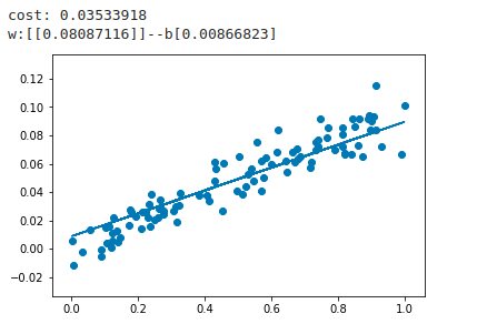
1
2
3
4
5
6
7
8
9
10
11
12
13
14
15
16
17
18
19
20
21
22
23
24
25
26
27
28
29
30
31
32
33
34
35
36
37
38
import kerasimport numpy as npimport matplotlib.pyplot as pltfrom keras.models import Sequentialfrom keras.layers import Densex_data = np.random.rand(100 ) noise = np.random.normal(0 ,0.01 ,x_data.shape) y_data = x_data*0.1 + noise plt.scatter(x_data,y_data) model = Sequential() model.add(Dense(units=1 , input_dim=1 )) model.compile (optimizer='sgd' ,loss='mse' ) for step in range (3000 ): cost = model.train_on_batch(x_data,y_data) if step == 100 : print ('cost:' ,cost) w,b = model.layers[0 ].get_weights() print ('w:{0}--b{1}' .format (w,b))y_predict = model.predict(x_data) plt.plot(x_data,y_predict) plt.show()
运行效果如下所示:
代码注解:
用来构建序列模型
用来添加神经网络的下一层结构
类似于穿件全连接的模型结构
对建立的模型进行编译,激活模型
model.train_on_batch(x_data,y_data) 开始对输入的数据和标签进行模型的训练
对于线性模型,我们只用了一层全连接的操作,默认使用了权值和偏置进行训练。
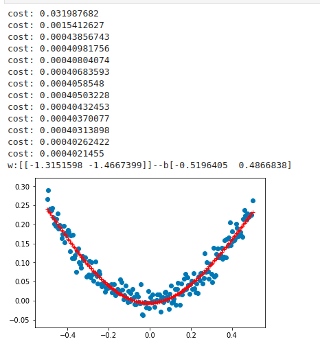
1
2
3
4
5
6
7
8
9
10
11
12
13
14
15
16
17
18
19
20
21
22
23
24
25
26
27
28
29
30
31
32
33
34
35
36
37
38
39
40
41
42
43
44
import keras import numpy as np import matplotlib.pyplot as pltfrom keras.layers import Dense,Activationfrom keras.models import Sequentialfrom keras.optimizers import SGDnx_data = np.linspace(-0.5 ,0.5 ,200 ) noise = np.random.normal(0 ,0.02 ,nx_data.shape) ny_data = np.square(nx_data)+noise plt.scatter(nx_data,ny_data) model = Sequential() model.add(Dense(units=2 , input_dim=1 )) model.add(Activation('tanh' )) model.add(Dense(units=1 , input_dim=2 )) model.add(Activation('tanh' )) sgd = SGD(learning_rate=0.3 ) model.compile (optimizer=sgd,loss='mse' ) for step in range (6001 ): cost = model.train_on_batch(nx_data,ny_data) if step % 500 == 0 : print ('cost:' ,cost) w,b = model.layers[0 ].get_weights() print ('w:{0}--b{1}' .format (w,b))y_predict = model.predict(nx_data) plt.plot(nx_data,y_predict,'r+' ) plt.show()
对于上面的非线性模型,我们使用了两层神经网络结构,使用的非线性函数为tanh作为激活函数,提示,非线性网络中必须使用,非线性激活函数,否则,模型输出只是线性的表达。